energies¶

Custom energies can be created by inheriting from javelin.energies.Energy and overriding the evaluate method. The evaluate method must have the identical signature and this gives you access to the origin and neighbor sites atom types and xyz’s along with the neighbor vector.

For example

class MyEnergy(Energy):
    def __init__(self, E=-1):
        self.E = E
    def evaluate(self,
                 a1, x1, y1, z1,
                 a2, x2, y2, z2,
                 neighbor_x, neighbor_y, neighbor_z):
        return self.E

This is slower than using compile classes by about a factor of 10. If you are using IPython or Jupyter notebooks you can use Cython magic to compile your own energies. You need load the Cython magic first %load_ext Cython. Then for example

%%cython
from javelin.energies cimport Energy
cdef class MyCythonEnergy(Energy):
    cdef double E
    def __init__(self, double E=-1):
        self.E = E
    cpdef double evaluate(self,
                          int a1, double x1, double y1, double z1,
                          int a2, double x2, double y2, double z2,
                          Py_ssize_t neighbor_x, Py_ssize_t neighbor_y, Py_ssize_t neighbor_z) except *:
        return self.E

class javelin.energies.DisplacementCorrelationEnergy(double J=0, double desired_correlation=NAN)¶

You can either set the desired_correlation which will automatically adjust the pair interaction energy (J), or set the J directly.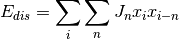

$E_{dis} = \sum_{i} \sum_{n} J_n x_i x_{i-n}$

>>> e = DisplacementCorrelationEnergy(-1)  # J = -1 produces a positive correlation
>>> e.evaluate(0, 1, 0, 0, 0, 0, 1, 0, 0, 0, 0)  # x1=1, y2=1
-0.0
>>> e.evaluate(0, 1, 0, 0, 0, 1, 0, 0, 0, 0, 0)  # x1=1, x2=1
-1.0
>>> e.evaluate(0, 1, 0, 0, 0, -1, 0, 0, 0, 0, 0)  # x1=1, x2=-1
1.0
>>> e.evaluate(0, 1, 1, 1, 0, 1, -1, -1, 0, 0, 0)  # x1=1, y1=1, z1=1, x2=1, y2=-1, z2=-1
0.3333333333333333

J¶: J: ‘double’ Interaction energy, positive J will creates negative correlations while negative J creates positive correlations

desired_correlation¶: The desired displacement correlation, this will automatically adjust the interaction energy (J) during the javelin.mc.MC execution to achieve the desired correlation. The starting J can also be specified

evaluate(self, int a1, double x1, double y1, double z1, int a2, double x2, double y2, double z2, Py_ssize_t target_x, Py_ssize_t target_y, Py_ssize_t target_z) → double¶

class javelin.energies.Energy¶

This is the base energy class that all energies must inherit from. Inherited class should then override the evaluate method but keep the same function signature. This energy is always 0.

>>> e = Energy()
>>> e.evaluate(1, 2, 3, 4, 5, 6, 7, 8, 9, 0, 1)
0.0

correlation_type¶: This is used when feedback is applied, 0 = no_correlations, 1 = occupancy, 2 = displacement. The desired_correlation must also be set on the energy for this to work.

evaluate(self, int a1, double x1, double y1, double z1, int a2, double x2, double y2, double z2, Py_ssize_t target_x, Py_ssize_t target_y, Py_ssize_t target_z) → double¶

This function always returns a double of the energy calcuated. This base Energy class always returns 0.

The evaluate method get passed the atom type (Z) and positions in the unit cell (x, y and z) of the two atoms to be compared, (atom1 is a1, x1, y1, z1, atom2 is a2, x2, y2, z2) and the neighbor vector (target_x, target_y, target_z) which is the number of unit cells that separate the two atoms to be compared

run(self, int64_t[:, :, :, ::1] a, double[:, :, :, ::1] x, double[:, :, :, ::1] y, double[:, :, :, ::1] z, Py_ssize_t[:] cell, Py_ssize_t[:, :] neighbors, Py_ssize_t number_of_neighbors, Py_ssize_t mod_x, Py_ssize_t mod_y, Py_ssize_t mod_z) → double¶

class javelin.energies.IsingEnergy(int atom1, int atom2, double J=0, double desired_correlation=NAN)¶

The Ising model

You can either set the desired_correlation which will

automatically adjust the pair interaction energy (J), or set the J directly.

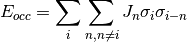
$E_{occ} = \sum_{i} \sum_{n,n\ne i} J_n \sigma_i \sigma_{i-n}$

The atom site occupancy is represented by Ising spin variables $\sigma_i = \pm1$ . $\sigma = -1$ is when a site is occupied by atom1 and $\sigma = +1$ is for atom2.

>>> e = IsingEnergy(13, 42, -1)  # J = -1 produces a positive correlation
>>> e.atom1
13
>>> e.atom2
42
>>> e.J
-1.0
>>> e.evaluate(1, 0, 0, 0, 1, 0, 0, 0, 0, 0, 0)  # a1=1, a2=1
-0.0
>>> e.evaluate(13, 0, 0, 0, 13, 0, 0, 0, 0, 0, 0)  # a1=13, a2=13
-1.0
>>> e.evaluate(42, 0, 0, 0, 13, 0, 0, 0, 0, 0, 0)  # a1=42, a2=13
1.0
>>> e.evaluate(42, 0, 0, 0, 42, 0, 0, 0, 0, 0, 0)  # a1=42, a2=42
-1.0

J¶: J: ‘double’ Interaction energy, positive J will creates negative correlations while negative J creates positive correlations

atom1¶

atom2¶

desired_correlation¶: The desired occupancy correlation, this will automatically adjusted the interaction energy (J) during the javelin.mc.MC execution to achieve the desired correlation. The starting J can also be specified

evaluate(self, int a1, double x1, double y1, double z1, int a2, double x2, double y2, double z2, Py_ssize_t target_x, Py_ssize_t target_y, Py_ssize_t target_z) → double¶

class javelin.energies.LennardJonesEnergy(double D, double desired, int atom_type1=-1, int atom_type2=-1)¶

The Lennard-Jones potential is a more realistic potential than javelin.energies.SpringEnergy that takes into account the strong repulsion between atoms as a close distance.

The Lennard-Jones potential is described by $E_{lj}$

$E_{lj} = \sum_{i} \sum_{n\ne i} D \left[\left(\frac{\tau_{in}}{d_{in}}\right)^{12} - 2 \left(\frac{\tau_{in}}{d_{in}}\right)^6\right]$

D is the depth of the potential well, $d$ is the distance between the atoms and $\tau$ is the desired distance (minimum energy occurs at $d = \tau$ ). Distances, $d$ and $\tau$ are in fractional coordinates.

(Source code, png, hires.png, pdf)

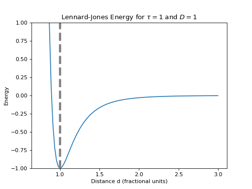
>>> e = LennardJonesEnergy(1, 1)  # D = 1, desired=1
>>> e.evaluate(0, 0, 0, 0, 0, 0, 0, 0, 1, 0, 0)  # target_x=1 ≡ d=1
-1.0
>>> e.evaluate(0, 0, 0, 0, 0, 0.5, 0, 0, 1, 0, 0)  # x2=0.5, target_x=1 ≡ d=1.5
-0.167876
>>> e.evaluate(0, 0, 0, 0, 0, 1, 0, 0, 1, 0, 0)  # x2=1, target_x=1 ≡ d=2
-0.031006
>>> e.evaluate(0, 0, 0, 0, 0, -0.5, 0, 0, 1, 0, 0)  # x2=-0.5, target_x=1 ≡ d=0.5
3968.0
>>> e.evaluate(0, 0, 0, 0, 0, 0, 0.5, 0, 1, 0, 0)  # y2=0.5, target_x=1 ≡ d=1.118
-0.761856

Optionally you can define a particular atom combination that only this energy will apply to. You can do this by setting atom_type1 and atom_type2 (must set both otherwise this is ignored). If the atoms that are currently being evaluated don’t match then the energy will be 0. It is suggested to include energies for all possible atom combinations in the simulation. For example

>>> e = LennardJonesEnergy(D=1, desired=1, atom_type1=11, atom_type2=17)  # Na - Cl
>>> e.evaluate(99, 0, 0, 0, 99, 0.5, 0, 0, 1, 0, 0)  # a1 = 99, a2 = 99
0.0
>>> e.evaluate(11, 0, 0, 0, 11, 0.5, 0, 0, 1, 0, 0)  # a1 = 11, a2 = 11
0.0
>>> e.evaluate(11, 0, 0, 0, 17, 0.5, 0, 0, 1, 0, 0)  # a1 = 11, a2 = 17
-0.167876
>>> e.evaluate(17, 0, 0, 0, 11, 0.5, 0, 0, 1, 0, 0)  # a1 = 17, a2 = 11
-0.167876
>>>
>>> e = LennardJonesEnergy(D=1, desired=1, atom_type1=17, atom_type2=17)  # Cl - Cl
>>> e.evaluate(99, 0, 0, 0, 99, 0.5, 0, 0, 1, 0, 0)  # a1 = 99, a2 = 99
0.0
>>> e.evaluate(11, 0, 0, 0, 11, 0.5, 0, 0, 1, 0, 0)  # a1 = 11, a2 = 11
0.0
>>> e.evaluate(11, 0, 0, 0, 17, 0.5, 0, 0, 1, 0, 0)  # a1 = 11, a2 = 17
0.0
>>> e.evaluate(17, 0, 0, 0, 17, 0.5, 0, 0, 1, 0, 0)  # a1 = 17, a2 = 17
-0.167876

D¶

atom_type1¶

atom_type2¶

desired¶

evaluate(self, int a1, double x1, double y1, double z1, int a2, double x2, double y2, double z2, Py_ssize_t target_x, Py_ssize_t target_y, Py_ssize_t target_z) → double¶

class javelin.energies.SpringEnergy(double K, double desired, int atom_type1=-1, int atom_type2=-1)¶

Hooke’s law for a simple spring can be used to describe atoms joined together by springs and are in a harmonic potential.

The spring energy is described by $E_{spring}$

$E_{spring} = \sum_{i} \sum_{n} k_n [d_{in} - \tau_{in}]^2$

$k$ is the force constant, $d$ is the distance between the atoms and $\tau$ is the desired distance (minimum energy occurs at $d = \tau$ ). Distances, $d$ and $\tau$ are in fractional coordinates.

(Source code, png, hires.png, pdf)

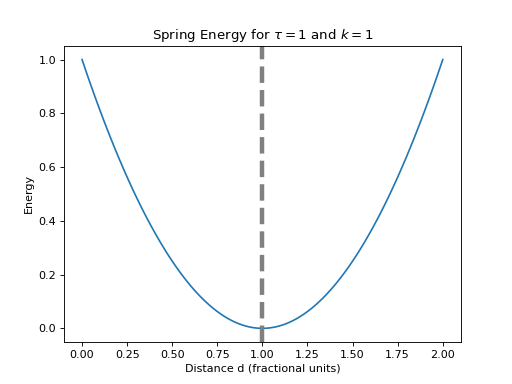
>>> e = SpringEnergy(1, 1)  # K = 1, desired=1
>>> e.evaluate(0, 0, 0, 0, 0, 0, 0, 0, 1, 0, 0)  # target_x=1 ≡ d=1
0.0
>>> e.evaluate(0, 0, 0, 0, 0, 0.5, 0, 0, 1, 0, 0)  # x2=0.5, target_x=1 ≡ d=1.5
0.25
>>> e.evaluate(0, 0, 0, 0, 0, 1, 0, 0, 1, 0, 0)  # x2=1, target_x=1 ≡ d=2
1.0
>>> e.evaluate(0, 0, 0, 0, 0, -0.5, 0, 0, 1, 0, 0)  # x2=-0.5, target_x=1 ≡ d=0.5
0.25
>>> e.evaluate(0, 0, 0, 0, 0, 0, 0.5, 0, 1, 0, 0)  # y2=0.5, target_x=1 ≡ d=1.118
0.013932

Optionally you can define a particular atom combination that only this energy will apply to. You can do this by setting atom_type1 and atom_type2 (must set both otherwise this is ignored). If the atoms that are currently being evaluated don’t match then the energy will be 0. It is suggested to include energies for all possible atom combinations in the simulation. For example

>>> e = SpringEnergy(K=1, desired=1, atom_type1=11, atom_type2=17)  # Na - Cl
>>> e.evaluate(99, 0, 0, 0, 99, 0.5, 0, 0, 1, 0, 0)  # a1 = 99, a2 = 99
0.0
>>> e.evaluate(11, 0, 0, 0, 11, 0.5, 0, 0, 1, 0, 0)  # a1 = 11, a2 = 11
0.0
>>> e.evaluate(11, 0, 0, 0, 17, 0.5, 0, 0, 1, 0, 0)  # a1 = 11, a2 = 17
0.25
>>> e.evaluate(17, 0, 0, 0, 11, 0.5, 0, 0, 1, 0, 0)  # a1 = 17, a2 = 11
0.25
>>>
>>> e = SpringEnergy(K=1, desired=1, atom_type1=17, atom_type2=17)  # Cl - Cl
>>> e.evaluate(99, 0, 0, 0, 99, 0.5, 0, 0, 1, 0, 0)  # a1 = 99, a2 = 99
0.0
>>> e.evaluate(11, 0, 0, 0, 11, 0.5, 0, 0, 1, 0, 0)  # a1 = 11, a2 = 11
0.0
>>> e.evaluate(11, 0, 0, 0, 17, 0.5, 0, 0, 1, 0, 0)  # a1 = 11, a2 = 17
0.0
>>> e.evaluate(17, 0, 0, 0, 17, 0.5, 0, 0, 1, 0, 0)  # a1 = 17, a2 = 17
0.25

K¶

atom_type1¶

atom_type2¶

desired¶

evaluate(self, int a1, double x1, double y1, double z1, int a2, double x2, double y2, double z2, Py_ssize_t target_x, Py_ssize_t target_y, Py_ssize_t target_z) → double¶